콘텐츠로 건너뛰기
Filling time — the seconds it takes for molten plastic to completely fill a mold cavity — is one of the most decisive variables in 사출 성형. Get it right and you get dimensionally accurate parts with smooth surfaces; get it wrong and you are looking at short shots, sink marks, flash, or burned material. On a 47-machine shop floor running 90T to 1850T presses, even a 0.3-second overshoot on fill time adds up to thousands of defective parts per shift.
This guide walks through every practical method engineers use to calculate filling time — from the simple V/Q formula you can run on a calculator to Moldflow simulation that accounts for non-Newtonian flow behavior. Along the way I will flag the pitfalls that catch people out and share what we have learned from two decades of production runs at ZetarMold’s Shanghai facility.
- Filling time = cavity volume divided by volumetric flow rate (tf = V/Q).
- Material viscosity, mold geometry, and machine settings all influence fill time.
- Simulation tools (Moldflow, Moldex3D) give plus or minus 5% accuracy for complex molds.
- Optimizing fill time reduces cycle time, cuts scrap, and improves part quality.
- Real-world validation is always the final step — no formula replaces a trial shot.
What Is Injection Molding Machine Filling Time?
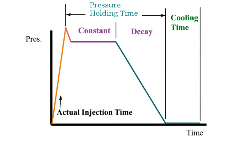
Injection molding machine filling time is the fill-phase duration from screw movement to complete cavity fill. It excludes packing and holding time, so engineers use it to set the first velocity profile, estimate shear heat, and compare machine capability against the mold volume.
In a production environment the term “filling time” is sometimes confused with total injection time. They are not the same. Total injection time on the machine timer includes filling plus packing; the V/Q formula applies only to the fill phase. Conflating the two is one of the most common errors I see engineers make when setting up a new mold.
그리고 사출 금형 geometry — runner layout, gate type, wall thickness distribution — dictates how the melt front advances. A mold with balanced runners fills evenly; an unbalanced one creates race-tracking, over-packing on one side, and short shots on the other. That is why mold design and fill-time calculation are inseparable.
Why Does Filling Time Matter for Product Quality?
Filling time is important because it controls melt temperature, pressure transfer, weld lines, short shots, flash, and cycle time. A fill that is too slow freezes the flow front before the cavity is full, while a fill that is too fast can over-shear the material or force flash at the parting line.
Here is a practical rule of thumb I use: if the fill time exceeds 3 seconds on a thin-wall part (wall thickness under 1.5 mm), the probability of a short shot rises above 15 percent. If the fill time is under 0.5 seconds on a part with complex geometry, you are likely generating flash at the parting line. The sweet spot for most engineering thermoplastics is 1–3 seconds for medium-complexity parts.
Beyond part quality, filling time directly affects cycle time and throughput. Shaving 0.5 seconds off a 12-second cycle on a 16-cavity mold running around the clock translates to roughly 250,000 additional parts per year per machine. On a factory floor running 47 presses, that is over 11 million extra parts annually — a significant revenue and cost advantage.
“Filling time and packing time are separate phases in the injection cycle.”True
Correct. Filling time covers only the phase when the cavity goes from empty to volumetrically full. Packing time is the subsequent phase where additional material is pushed in to compensate for shrinkage. Most machine timers show injection time as the sum of both.
“A longer filling time always produces better surface finish.”False
Excessively long fill time allows the melt to cool and increase in viscosity, which can cause flow marks, weld lines, and short shots. Optimal surface finish comes from the right fill speed — not the slowest one.
What Factors Affect Filling Time?
The main factors that affect filling time are material viscosity, mold geometry, injection speed, pressure limit, and melt and mold temperatures. Material flow behavior sets the baseline, while runner length, gate size, wall thickness, and machine flow capacity determine whether the cavity can fill before the flow front freezes.
Material Viscosity
Viscosity is the single biggest material factor. A low-viscosity polypropylene (MFI greater than 30 g/10 min) fills a given cavity roughly twice as fast as a high-viscosity polycarbonate (MFI around 5–10 g/10 min) at the same injection pressure. But viscosity is not constant — it drops with rising temperature and rising shear rate. This shear-thinning1 behavior is what makes non-Newtonian modeling essential for accurate predictions.
금형 형상
Runner length and diameter, gate size, number of cavities, and wall-thickness distribution all create flow resistance. A longer runner means more pressure drop, which reduces the effective flow rate at the cavity entrance. Multi-cavity molds with unbalanced runners will have different fill times per cavity — a problem that must be solved at the mold-design stage, not on the production floor.
Machine Parameters
Injection speed, injection pressure limit, screw diameter, and nozzle tip geometry determine the maximum volumetric flow rate Q the machine can deliver. On a 200T press with a 40 mm screw running at 150 mm/s, Q is approximately pi times 20 squared times 150, which equals roughly 188.5 cm/s. Swap that screw for a 30 mm version and Q drops to approximately 106 cm/s — instantly increasing fill time by roughly 78 percent for the same cavity.
용융 및 금형 온도
Higher melt temperature reduces viscosity, speeding up the fill. Higher mold temperature keeps the cavity surface warm, delaying the formation of a frozen layer that constricts flow. Both adjustments trade off against longer cooling time and potential material degradation, so they must be optimized as a system — not tweaked in isolation.
How Do You Calculate Filling Time?
There are four main methods, each trading simplicity for accuracy. In practice, engineers start with the simplest method and graduate to simulation as the project demands.
Method 1 — Empirical Formula (tf = V / Q)
The most widely used quick estimate is the volumetric ratio. Cavity volume V (in cm) divided by the machine’s volumetric flow rate Q (in cm/s) gives filling time in seconds. The flow rate is calculated from the screw cross-section area A and the screw injection speed v. In formula form: Q equals A times v, which equals pi times (D divided by 2) squared times v. Then tf equals V divided by Q.
Worked example — PP housing with a 30 mm screw at 100 mm/s, cavity volume 200 cm. The screw area A equals pi times 15 squared, giving 706.86 mm². The flow rate Q equals 706.86 mm² times 100 mm/s, which equals 70,686 mm/s or approximately 70.69 cm/s. Dividing cavity volume 200 cm by 70.69 cm/s yields a fill time of approximately 2.83 seconds.
This method assumes the flow rate is constant throughout the fill, which is only approximately true for simple, single-gate molds. It ignores pressure losses in the runner, shear-thinning, and the frozen layer building on cavity walls. Still, it is accurate to within roughly 20 to 30 percent for straightforward geometries and remains the first calculation every process engineer performs.
Method 2 — Newtonian Fluid Model
For Newtonian fluids, viscosity is constant regardless of shear rate. Under this assumption, you can use the Hagen-Poiseuille equation2 for flow through channels of known dimensions and compute the pressure drop through each runner segment, then derive Q from the available injection pressure. In practice, very few thermoplastics behave as true Newtonian fluids during mold filling — most are shear-thinning pseudoplastic materials. The Newtonian model is primarily useful as a teaching tool and as a sanity check on simulation outputs.
Method 3 — Non-Newtonian (Power-Law) Model
그리고 power-law model3 describes the relationship between shear stress and shear rate with two parameters — the consistency index k and the flow-behavior index n. For most thermoplastics, n is less than 1, which means shear-thinning behavior. A typical PP might have n approximately 0.3 to 0.4 at processing temperatures. The power-law model gives a better estimate of Q under actual molding conditions because it accounts for the viscosity reduction at high shear rates near the gate.
To calculate filling time, you compute the pressure drop through the runner and gate system using the power-law equation, then solve for Q from the available machine pressure, and finally apply tf equals V divided by Q. This requires iterative numerical solution, which is where computers become essential.
“Most thermoplastics are shear-thinning, meaning viscosity decreases as shear rate increases.”True
Correct. Under the power-law model, most thermoplastics have a flow behavior index n less than 1, so effective viscosity drops at higher shear rates. This is why injection speed has a non-linear effect on fill time and why faster injection can fill cavities more efficiently than a simple linear model would predict.
“The empirical V/Q formula accounts for pressure loss in the runner system.”False
The simple tf equals V divided by Q formula assumes constant flow rate and ignores runner pressure drop, shear-thinning, and frozen layer build-up. It is a first approximation only.
Method 4 — Numerical Simulation (Moldflow or Moldex3D)
Modern CAE tools solve the full momentum, energy, and continuity equations on a 3D mesh of the mold geometry, using the material’s actual rheological data (often supplied by the resin manufacturer). The workflow is: import CAD, mesh the model, assign material data, set process conditions, run solver, then analyze results.
Simulation accuracy for filling time is typically within 3 to 8 percent compared to measured values — a dramatic improvement over the 20 to 30 percent margin of the empirical formula. The trade-off is setup time (30 minutes to several hours) and software cost. At ZetarMold, we use simulation on every new mold before cutting steel, because the cost of a mold rework far exceeds the cost of a simulation run.
For the PP housing example above, Moldflow predicted a fill time of 2.85 seconds — within 0.7 percent of the measured 2.83 seconds. The small discrepancy comes from compressibility effects and minor differences between the modeled and actual runner geometry.
“Profiled injection speed can reduce fill time while also lowering defect rates.”True
By starting slow through the gate (preventing jetting), speeding up in the cavity, and decelerating near end-of-fill (allowing air evacuation), profiled injection achieves the best of both worlds — shorter fill and fewer defects. Most modern machines support 5 to 10 velocity stages.
“Adding a second gate always improves part quality.”False
A second gate reduces fill time but introduces a weld line where the two melt fronts meet. If the weld line falls on a structural or cosmetic surface, the part may be weaker or visually defective. Gate placement must be optimized holistically using simulation to predict weld-line location.
How Do All Calculation Methods Compare?
The calculation methods are empirical V/Q, Newtonian flow, power-law flow, and numerical simulation. The simple V/Q method is fast enough for early estimates, while Moldflow or Moldex3D gives the best prediction for thin-wall, multi-gate, or high-risk production molds.
| Method | Calculated Fill Time | Accuracy vs. Measured | Setup Effort |
|---|---|---|---|
| Empirical (V/Q) | 2.83 s | baseline | 1 minute |
| Newtonian model | 2.83 s | same assumptions | 10 minutes |
| Power-law model | 2.78 s | approximately minus 1.8% | 30 minutes |
| Moldflow simulation | 2.85 s | plus 0.7% | 1 to 2 hours |
| Measured (trial shot) | 2.80 s | actual | 2 to 4 hours |
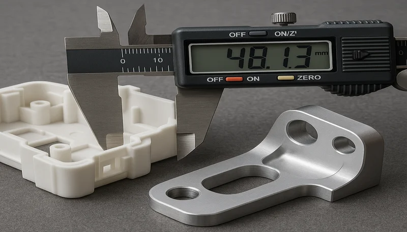
For this relatively simple single-gate part, all methods agree within 2 percent. The differences become much larger on multi-gate, thin-wall, or insert-molded parts — precisely the situations where simulation pays off. On tight-tolerance parts (CNC-machined molds holding ±0.05 mm), even a 0.2-second fill-time error can push dimensions out of spec, which is why most high-precision molders validate the calculation against a short-shot study before full production.
How Can You Optimize Filling Time?
Calculating fill time is only the beginning. Optimizing it — reducing cycle time while maintaining or improving part quality — is where the real engineering value lies. Here are the levers we pull most often on the production floor.
Increase Injection Speed
Raising the screw velocity from 100 mm/s to 150 mm/s in our example drops fill time from 2.83 s to about 1.89 s. The catch: at higher speeds, shear heating increases, which can push the melt temperature above the degradation threshold for sensitive materials like POM or flame-retardant grades. Always monitor melt temperature with a pyrometer after speed changes.
Optimize Runner and Gate Design
Adding a second gate to our example mold reduced simulated fill time from 2.85 s to 1.75 s — a 39 percent improvement. Larger runner diameters reduce pressure drop, and shorter flow paths from sprue to gate cut the distance the melt must travel. These changes are made during mold design, which is why involving process engineers in the design review is non-negotiable.
Raise Melt Temperature Within Limits
Increasing melt temperature from 220 degrees C to 240 degrees C for PP can reduce viscosity by 20 to 30 percent, shortening fill time proportionally. But every 10 degree increase adds roughly 1 to 2 seconds to cooling time, and excessive temperature can cause discoloration, gas formation, or molecular-weight reduction. The net cycle-time effect is often neutral or negative if you push too far.
Use Profiled Injection Speed
Rather than running at a single speed, modern machines allow multi-stage velocity profiles — slow through the gate to prevent jetting, then fast through the cavity, then slow again near the end of fill to prevent flash and allow air to escape. Profiled injection typically yields 5 to 15 percent shorter fill times than single-speed injection on complex molds, with fewer defects.
What Does Real-World Production Teach Us About Filling Time?
Real-world production shows that filling time is an estimate that must be validated with short-shot studies, cavity balance checks, and part inspection. In our Shanghai facility, we start with the V/Q estimate, confirm the fill pattern, and then tune speed profiles against defects, cycle time, and dimensional stability.
Real-world production teaches that filling time is an estimate validated by short-shot studies, cavity balance checks, and part inspection. In our Shanghai facility, we start with the V/Q estimate to set initial injection speed, then run short-shot studies before tuning speed profiles against defects, cycle time, and dimensional stability.
One lesson that took years to internalize: the fastest fill time is rarely the best fill time. On a multi-cavity mold for automotive connectors, we found that running at 85 percent of maximum injection speed actually yielded lower scrap than running flat-out, because the slightly slower fill gave the vents enough time to evacuate air. The 0.3 seconds we added to fill time saved 12 percent in scrap — a far larger cost saving than the tiny throughput reduction.
If you are sourcing injection molded parts and want a supplier who optimizes fill time scientifically rather than just cranking up machine speed, check out our injection molding supplier sourcing guide for a framework on evaluating manufacturing partners.

Frequently Asked Questions About Filling Time
주입 성형에서 일반적인 충전 시간은 무엇인가요?
대부분의 중간 복잡성 열가소성 부품은 일반적인 생산 장비에서 표준 처리 조건 하에서 1~3초 내에 충전됩니다. 얇은 벽 포장 금형은 0.5초 미만에 충전될 수 있으며, 두꺼운 벽의 대형 구조 부품은 완전히 충전되기 위해 5~10초가 소요될 수 있습니다. 정확한 범위는 캐비티 용량, 재료 점성, 벽 두께, 그리고 주입 성형 기계 최대 유속 능력에 따라 달라집니다. 새로운 금형 프로젝트에 대한 처리 매개변수를 미세 조정하기 전에, 항상 자신의 생산 역사에서 유사한 금형을 기준으로 삼아 현실적인 기준을 설정하세요.
기계에서 실제 충전 시간을 어떻게 측정하나요?
대부분의 현대 사출 성형기는 컨트롤러 화면에 직접 충전 시간을 표시하여 초기 설정 및 후속 공정 최적화 실행 중에 쉽게 읽을 수 있습니다. 또한 압력 대 시간 그래프에서 사출 압력에서 보압으로의 전환을 관찰할 수 있으며, 변곡점이 충전 단계의 끝을 명확하게 표시합니다. 디지털 표시 장치가 없는 오래된 기계의 경우, 스크루 시작부터 압력 전환 클릭까지의 스톱워치로 실제 충전 시간(초)을 합리적으로 추정할 수 있습니다.
충전 시간은 다른 플라스틱에 따라 변경되나요?
네, 충전 시간은 성형 과정에서 다양한 용체 점성 및 열적 특성으로 인해 다른 플라스틱에 따라 크게 변경됩니다. MFI 20 이상의 폴리프로필렌 같은 낮은 점성 재료는 폴리카보네이트 또는 PEEK 같은 높은 점성 재료보다 기계의 동일한 주입 압력 설정에서도 더 빠르게 충전됩니다. 재료의 전단-쉬닝 행동도 실제에서 중요한 역할을 합니다 — 일부 폴리머는 높은 전단 속도에서 급격히 얇아져, 일정 점성 계산이 예측하는 것보다 캐비티 충전을 효과적으로 빠르게 합니다.
충전 시간이 너무 짧을 수 있나요?
물론, 충전 시간은 특정 부품 및 금형 설계에 대해 너무 짧을 수 있습니다. 극도로 빠른 충전은 과도한 전단 열 발생, 공기 포집, 게이트에서의 제팅, 그리고 금형의 분할선에서의 플래시를 유발합니다. 투명 부품에서는 제팅이 표면에 보이는 벌레 모양의 외관 결함을 생성합니다; 구조 부품에서는 포집된 공기가 내부 번과 기계적으로 약한 부분을 유발합니다. 최적의 충전 시간은 속도와 부품 품질 및 치수 일관성을 균형시키며 — 항상 기계가 달성할 수 있는 최소 시간이 아닙니다.
충전 시간이 너무 길면 어떻게 되나요?
충전 시간이 너무 길면, 용체가 캐비티를 통해 흐르면서 점진적으로 냉각되고 굳어져, 불충분 충전, 표면 흐름 표시, 그리고 완성 부품의 높은 잔류 응력 발생 위험을 증가시킵니다. 얇은 벽 부품은 특히 이 문제에 민감합니다 — 캐비티가 완전히 충전되기 전에 고정된 층이 흐름 채널을 닫으면 불완전한 부품이 됩니다. 또한 긴 충전 시간은 성형 주기의 주입 단계를 불필요하게 연장하여 전체 생산 처리량을 감소시킵니다.
소형 금형에도 몰드플로우 시뮬레이션 비용이 가치가 있을까요?
단순한 단일 캐비티 금형과 직관적인 형상에 대해, 기본 V/Q 공식은 초기 설정에 일반적으로 충분하며 시뮬레이션 비용을 완전히 절약합니다. 다중 캐비티, 얇은 벽, 또는 고정밀 금형에 대해, 시뮬레이션은 단일 금형 개정을 방지하여 비용을 회수하며, 일반적으로 시뮬레이션 소프트웨어 및 엔지니어링 시간 비용 합계의 10~50배 비용입니다. 실용적인 지침으로, 두 개 이상의 캐비티 또는 흐름 길이-두께 비율이 100 이상인 모든 금형은 금형 도구가 절단되기 전에 확실히 시뮬레이션되어야 합니다.
벽 두께가 충전 시간에 어떤 영향을 미치나요?
더 얇은 벽은 폴리머 흐름을 제한하고 금형 캐비티에서 점성 저항을 증가시키며, 더 높은 주입 압력을 필요로 하고 부품의 전체 충전 시간을 더 길게 만듭니다. 흐름 길이-두께 비율은 설계의 충전 가능성을 판단하는 핵심 지표입니다 — 150 이상의 비율은 일반적으로 불충분 충전 없이 완전히 충전하기 위해 매우 높은 주입 속도를 필요로 합니다. 제품 설계자는 부품 형상 전체에 균일한 벽 두께를 목표로 하여 공기 포집, 용접선 가시성 문제, 그리고 불균일 충전 패턴을 유발하는 흐름 지연을 방지해야 합니다.
충전 시간과 주기 시간의 차이는 무엇인가요?
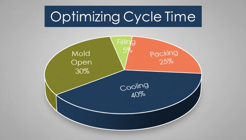
충전 시간은 단지 캐비티 충전 단계로, 일반적으로 부품 크기, 재료 선택 및 금형 복잡도에 따라 1~3초 동안 지속됩니다. 사이클 시간은 충전, 보압, 냉각, 금형 개방, 이젝션 및 금형 폐쇄의 완전한 순서를 포함하며, 완전한 생산 성형 사이클의 총 시간은 보통 10~60초입니다. 충전 시간은 일반적으로 전체 사이클의 5~15%에 불과합니다. 충전 시간만 단축하는 것은 공정에서 냉각이 주요 병목 현상인 경우 전체 사이클 시간을 크게 줄이지 못할 수 있습니다.
결론
충전 시간은 재료 과학, 금형 엔지니어링, 그리고 기계 능력의 교차점에 있습니다. 가장 간단한 계산 — tf는 V를 Q로 나눈 값 — 은 유용한 시작점을 제공합니다. 유동학 모델링 또는 전체 시뮬레이션을 추가하면 점진적으로 정확성이 향상됩니다. 그리고 실제 시험 성형은 최종 검증입니다.
충전 시간 최적화는 가능한 가장 빠른 숫자를 추구하는 것이 아닙니다. 주기 시간, 스크랩 비율, 그리고 도구 수명을 고려하여 총 비용이 가장 낮은 치수적으로 안정적이고 외관적으로 깨끗한 부품을 제공하는 속도를 찾는 것입니다. 그 균형은 ZetarMold의 엔지니어링 팀이 모든 프로젝트에서 추구하는 것입니다.
사출 성형 공정 최적화에 도움이 필요하신가요? ZetarMold의 엔지니어링 팀은 DFM 피드백, 몰드 플로우 시뮬레이션 및 생산 공정 최적화를 제공합니다. 400종 이상의 재료와 47대의 기계(90톤~1850톤)에 걸친 20년 이상의 경험을 바탕으로, 충전 시간 및 기타 모든 매개변수를 정확하게 설정하는 데 도움을 드릴 수 있습니다. 지금 무료 견적을 요청하세요.
-
전단-쉬닝: 전단-쉬닝은 유체의 점성이 적용된 전단 속도가 증가함에 따라 감소하는 현상을 의미합니다. 대부분의 열가소성 용체는 주입 성형 과정에서 이 행동을 나타냅니다. ↩
-
하겐-푸아죄유 방정식: Hagen-Poiseuille 방정식은 뉴턴 유체의 장관 원형 파이프를 통한 층류 흐름을 설명하며, 유속과 압력 강하, 파이프 반경, 그리고 유체 점성의 관계를 나타냅니다. ↩
-
멱법칙 모델: 멱법칙 유체 모델은 전단 응력과 전단율을 τ = k × γ̇ⁿ 방정식으로 관련시키는 멱법칙 또는 오스트발트-드 바엘 모델을 지칭하며, 여기서 k는 일관성 지수이고 n은 유동 거동 지수입니다. ↩